|
|
|
|
|
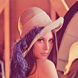
Notes 0004Image FiltersLast class we talked about point processing - image manipulation by changing the values/colors of individual pixels. Today we'll be discussing more general forms of image filtering. ConvolutionWithout going too deeply into the idea, a convolution is just a weighted sum of two images. Usually, one of the images is much smaller, and is called the `filter', or `kernel'. After the convolution operation, the resulting image has the desired properties `indicated' by the `kernel'. (A more complicated view is that the resulting image is a correlation between the input image and the filter.) Before we get into the details of actually applying the filter, lets look at a few examples first. Throughout this whole document, we'll be looking at filters of the standard `lena' image (this image is used to judge the performance of image compression, image filters, watermarking, etc., schemes):
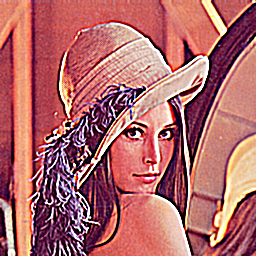
Now, lets move onto the filters, and the transformed image under those filters.
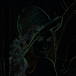
Notice in the first three images, that as the central value (in the kernel) gets higher, the image becomes less and less blury. Intuitively, that's because you're giving more and more `weight' to the central pixel (more of the value of the final pixel is coming from the pixel itself and not from the neighbours). Can you guess what effect this following kernel will have?
A quick way to experiment with these values is to use Photoshop; in Filters|Other|Custom, and you just type in the matrix that you think will make some effect happen. You can also implement relatively simple code and do these things yourself in a program. How does it actually work?And now, lets get to the idea of how it actually works. Usually, the very first thing we do is normalize the kernel. That means a
loop that looks sort of like this:
Basically since this is a weighed `sum' we're interested in, the effect of `multiplying' our image by the kernel has to leave the image at the same brightness level. For example, if the kernel is higher than 1, then the image will tend to get brighter (in addition to getting the effect of the kernel), and if it's lower than 1, then the image will tend to get darker.
Once we have the kernel, it is just a matter of (pseudo code):
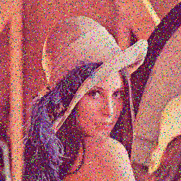
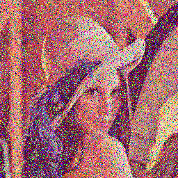
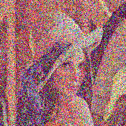
Note that this is pseudo code (eventhough it may look like C). An important thing to notice is that image[y+u][x+v], considering that you're starting with x,y equal to 0, and the u,v start out negative, you might actually end up with a negative index. These are the things the implementation has to watch out for - but logically, the code above works. This notion of borders is actually serious. There is no good way of handling it. One way is to just ignore the border pixels altogether. Another way is to wrap around the image (the bottom gets wrapped around to the top, etc.). You can also create a new normalized kernel that only includes the `available' pixels. One point that hasn't been mentioned but which deserves some attention, is that convolution is `never' implemented as above. Just think, if you have a kernel of 3x3, that's 9 multiplications per image pixel. If you have an image of 1024x1024, you're talking about on the order of 9 million multiplications just to apply an image filter. That would be slow. Usually, convolution is implemented as a Fast Fourier Transform (FFT). The trick is that multiplication of frequency cooficients in frequency domain is the same as a convolution in the spacial domain (we'll get to that a bit later when we deal with signals). The interesting thing turns out that convolution is actually just like multiplication, and in fact most large number (100s of digits) libraries perform multiplication by first applying the FFT, then multiplying individual cooficients, then doing an inverse transform, to get the result of multiplication. Other Spacial FiltersMedian FilterMedian Filter is especially useful in removing noise from an image. Here's an example:
As you can see, the filter recovers an image quite nicely (well, the recovered image is a bit blury). The median filter just involves this: choose a bunch of pixel values, sort them, take their median, and that's it. More precisely, there is also a `kernel' that indicates which pixels should be used in figuring out the median. If the `kernel' is:
Then all the pixels are used in the median calculation, if the kernel is:
Then only those pixels that fall under a `1' are used. The procedure (similar in loops to convolution) goes this way: whenever you see a pixel that falls under a 1, you write it to an array. You then sort that array, and the median is the new pixel value. That's it. Many times, the median kernels try to be `circular', so very often kernels have 0s on the edges. Things in class about image warping; distortions, etc., as well as image generation.
|